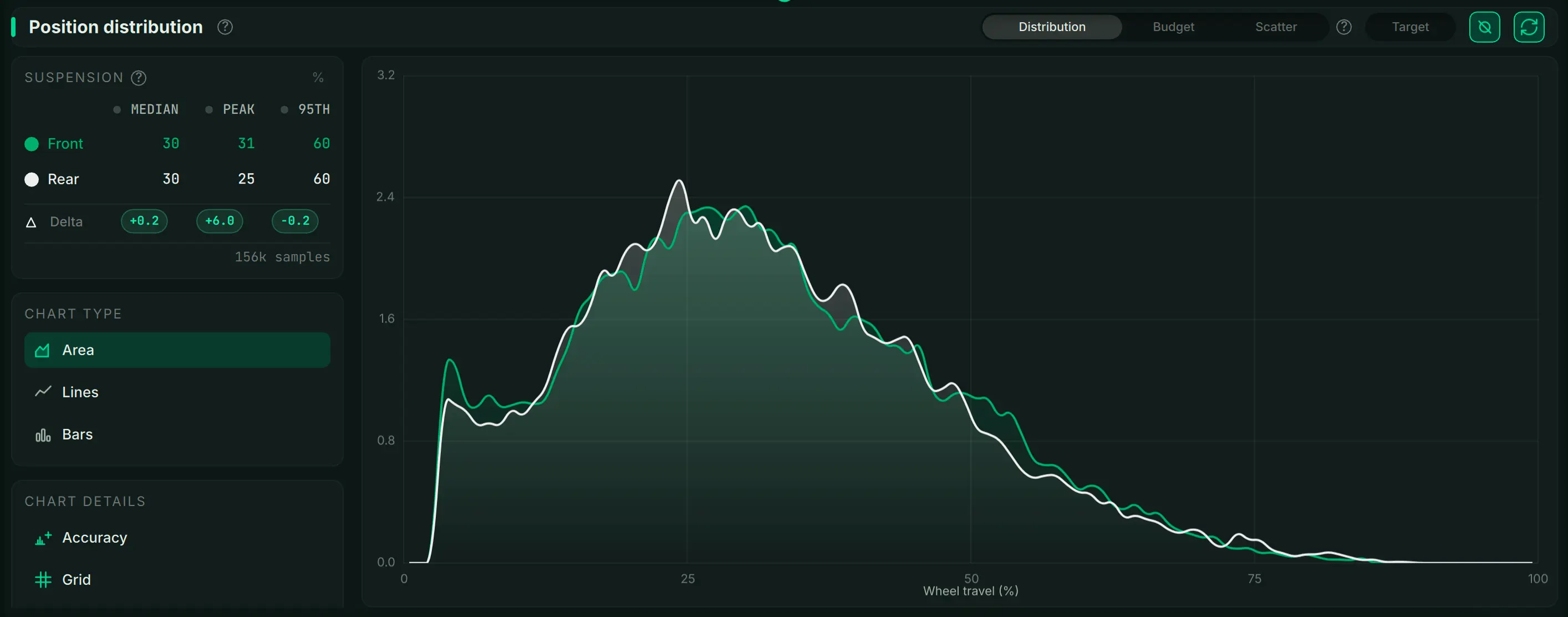
A travel histogram is a bar chart with two axes. The horizontal axis is suspension position, from fully open on the left to bottom-out on the right, usually as a percentage of total travel. The vertical axis is time — how long the suspension sat at each position during the run.
Each bar answers one question: how often did the fork or shock live here? Tall bars mark the positions your suspension used most, and the overall shape — not any single bar — tells you whether the setup supports you or swallows the stroke.
The chart is only as honest as the data behind it. A linear sensor on the fork and another on the shock report shaft position hundreds of times per second, and the logger time-stamps every reading. The BYB Telemetry software then maps shaft movement to wheel travel using your frame's leverage ratio and sorts the samples into the histogram.
A typical BYB Telemetry V3 session feeds the histogram from these channels:
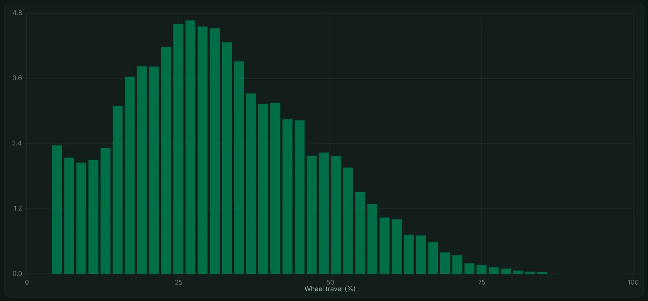
Start with the location of the tallest bars, then read the tails. A peak centred on your dynamic sag — around 30% travel for many trail bikes — signals a balanced chassis that resists diving yet stays active. That is usually the target shape.
A peak sitting deep, past 50% travel, means the spring is too soft or lacks support, so the bike rides low and loses reserve travel for big hits. A peak stuck shallow, below 20%, means the setup is too firm and never reaches its mid-stroke, so the ride feels harsh over small chatter.
The right-hand tail matters as much as the peak. A small cluster of bars at full travel is healthy and shows you use the whole stroke; a large spike at 100% means repeated bottom-outs, a cue to add pressure or a volume spacer.
Read the fork and shock histograms together. If one end peaks at sag while the other sits deep, the bike is unbalanced front to rear, and that imbalance — not a single component — is what you correct first.
Example — a rider sees a rear travel histogram peaking at 20% travel with almost no bars past mid-stroke, a classic over-firm signature. Dropping shock pressure from 200 PSI to 185 PSI shifts the peak toward 30% sag and fills in the mid-stroke, confirming fuller use of the stroke. The values are illustrative.
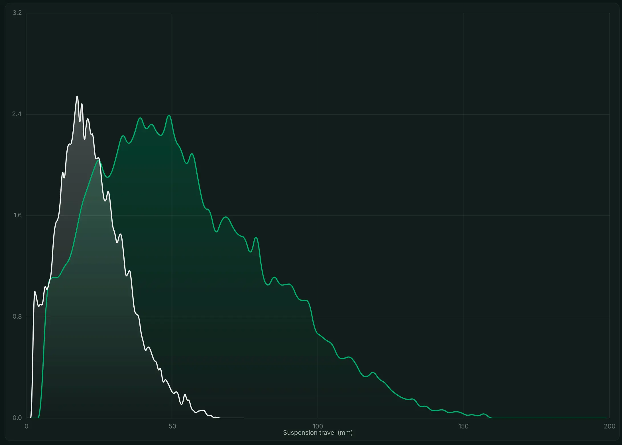
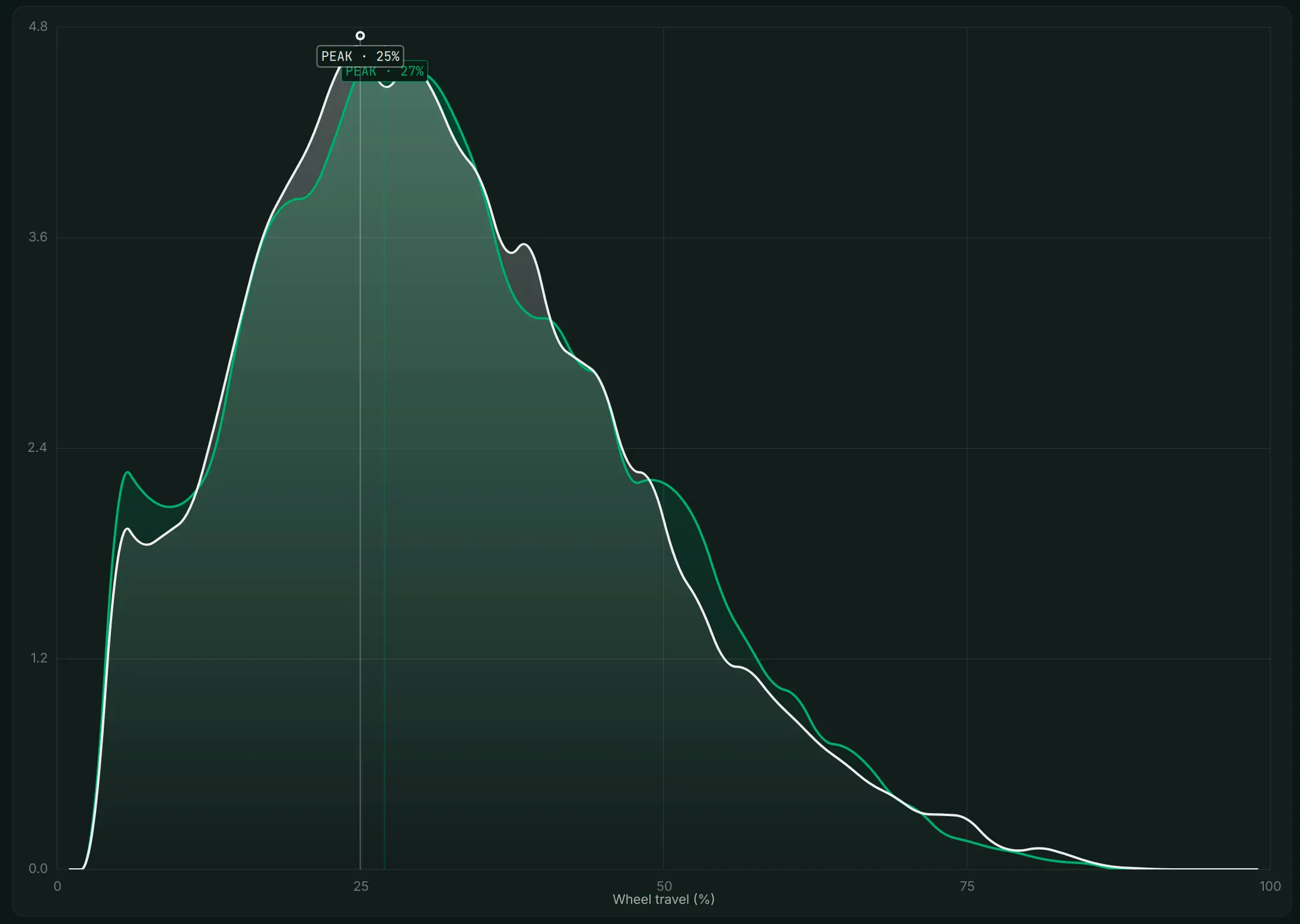
A histogram is fastest to read as a short, fixed routine, and data acquisition MTB telemetry rewards that consistency. Run the same steps every session so the shapes stay comparable across changes.
This measure, change one thing, re-measure loop is the backbone of honest suspension tuning. To capture these histograms on your own bike, Explore the BYB Telemetry Kit and review the full sensor package.
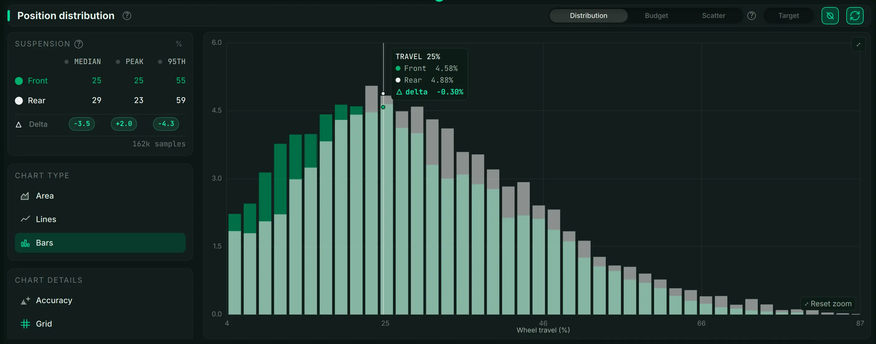
A single clear peak near your dynamic sag, roughly 30% travel, with a short tail that reaches full travel only a few times per run. That shape shows support in the mid-stroke and full use of the available stroke.
A twin-peak shape usually means two very different terrain types in one run, or a harsh transition in the damper tune. Split the data by trail segment before reading it.
One clean reference run is enough to spot the peak, but two or three repeats of the same segment average out rider variation and make the shape trustworthy.